Alongside applying for jobs and also taking courses on Python and SQL, I’ve been practicing some Data Wrangling and Data Visualization Skills using dplyr and ggplot2. The Data set I’ve used was Downloaded as a .csv File from Kaggle. The dataset contains 21 different variables, however not all 21 were used. The Horror Movies Dataset contains 21 columns and contains about 32,540 movies. However, after filtering for only English movies and already released movies, about 21,000 movies remain. The file I used to wrangle the data is available on my GitHub.
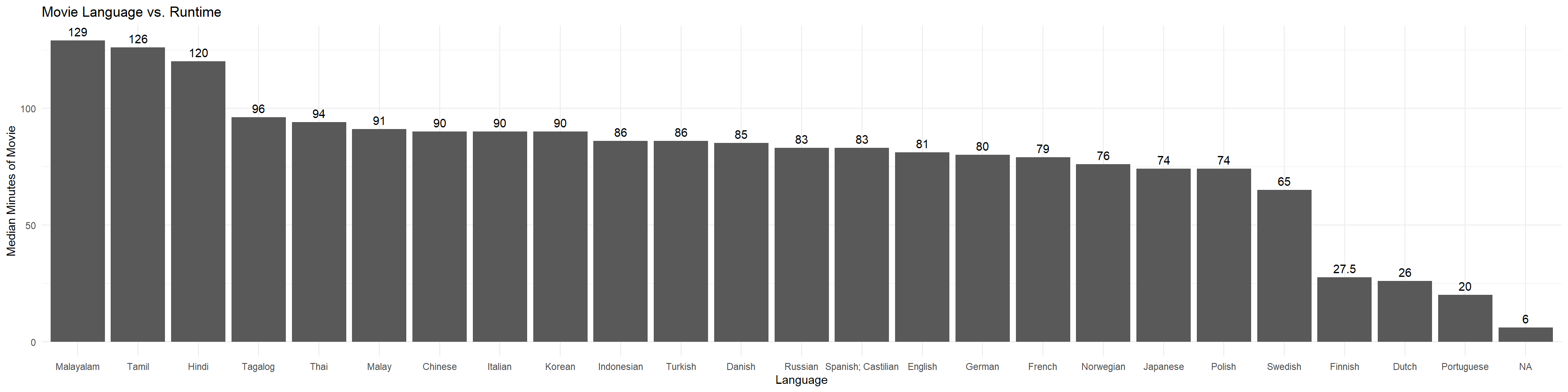
The first tidbit of insights I noticed was examining the relationship between the languages of the movies against the median run times. The number of movies for each language ranges from 51 (Polish) to 20,757 (English). The languages with the highest median movie run times all originate from the Indian Subcontinent. These languages are Malayalam, Tamil, and Hindi. English language movies are more around the middle with a median run time of about 81 minutes.
Moving forward in the post, all charts are populated with filters on English movies and Released Movies.
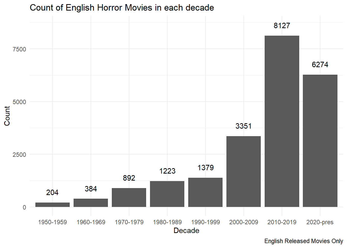
Using Case When statements, I categorized the release years by decade. The above chart contains how many English Released Movies are in the Horror Movies Dataset by decade. The release of horror movies rapidly increased in the 21st Century, with 2010-2019 having more released movies than 1950-2009 combined. Furthermore, we’re just 3 years into the current decade and 6,274 horror movies have been released. At this rate, the number of Horror Movies released this decade will be double than 2010-2019.
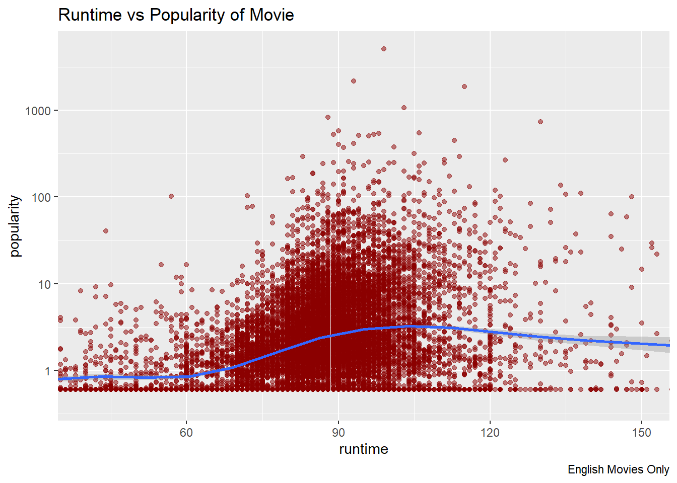
One of the questions I had while poring through the data set was if there was a relationship between the run time of the movie and its popularity. I transformed popularity using a log10 base transformation and applied a smoothed line to the chart above. I noticed that movie popularity increased when a movie’s run time was between 60 minutes and 105 minutes. However, movies with a movie run time over 115 minutes started to see their popularity stay stagnant.
Many of the horror movies also have other genre tags along with the horror tag. In the table below, for example, the movie Nope has three other genres; Mystery, Science Fiction, and Thriller.
en_movies %>%
  select(title, genre_names) %>%
  head()
## # A tibble: 6 × 2
##   title                    genre_names
##   <chr>                    <chr>
## 1 Orphan: First Kill       Horror, Thriller
## 2 Beast                    Adventure, Drama, Horror
## 3 Smile                    Horror, Mystery, Thriller
## 4 The Black Phone          Horror, Thriller
## 5 Jeepers Creepers: Reborn Horror, Mystery, Thriller
## 6 Nope                     Horror, Mystery, Science Fiction, Thriller
I wrangled the English horror movie Data set using several case when statements to create dummy variables. In layman’s terms, I separated genre_names into individual genre columns, each with a 1 if the genre is present and a 0 if it isn’t.
The heat map below shows a heat map of genre proportions by decade. Here’s an example on how to read the heat map :
24% of Horror Movies released between 2020 and the present include “Thriller” as a genre
(I sure hope that makes it easier to read!).
With that, here are a few observations I noticed:
- 53% of Horror Movies were also Science Fiction between 1950-1950. However, the share of Science Fiction Movies declined to only 7% today.
- Horror and Thriller really go hand in hand. Horror-Thriller movies make up a sizable number in each decade.
- Comedy Movies are on the rise! 17% of horror movies from 2020 to the present are Horror-Comedy movies and that share has been slowly increasing.
The chart above is interactive, so feel free to play around and see if you can pull any insights as well!